Oil and Gas Production Prediction

Background

As the world's primary fuel sources, oil and natural gas are major industries in the energy industry and have a significant impact on the global economy. Oil and gas production and distribution processes and systems are very complicated, capital-intensive, and require cutting-edge technology. Because of the production process or upstream part of the industry, natural gas has historically been connected to oil.Natural gas has been regarded as a nuisance for much of the industry's history. As a result of shale gas development in the United States and its lower greenhouse gas emissions when combusted when compared to oil and coal, natural gas has taken on a more major position in the world's energy supply.Typically, the industry is divided into three categories:Oil and gas exploration and production are classified as upstream; transportation and storage are classified as midstream; and refining and marketing are classified as downstream.Water is central to all activities of the oil and gas industry.

Oil and gas prices have a direct and indirect impact on the domestic economy, with oil and gas prices affecting the overall health of the economy. Individuals and businesses all across the world rely heavily on oil and gas. There are numerous challenges throughout the process like resource management, volatility of prices, environmental footprint, controlling all stages of water cycle and other industrial challenges.

The process of extracting hydrocarbons and sorting the mixture of liquid hydrocarbons, gas, water, and particles, removing non-saleable ingredients, and selling the liquid hydrocarbons and gas is known as production. Crude oil from many wells is frequently handled at production sites.One of the most pressing issues in the oil and gas sector is forecasting oil production.

Importance of Oil and Gas Production Prediction

Estimating the amount of liquid that a well could generate over its lifetime is critical, particularly from an economic and business standpoint. The well site, geological considerations, drilling technology utilized by the operator drilling, and nearby wells and their effects on each other are all aspects that play a role.

Objective

The objective is to Use Machine Learning to predict production for a certain well. Given a well's production curve, one should be able to create a label and use well features to create an ML model that estimates oil production. Engineering characteristics, geological features, and location features are all possible well features.

Relevance of Xceed

Xceed Analytics provides a single integrated data and AI platform that reduces friction in bring data and building machine models rapidly. It further empowers everyone including Citizen Data Engineers/Scientist to bring data together and build and delivery data and ml usecases rapidly. It's Low code/No code visual designer and model builder can be leveraged to bridge the gap and expand the availability of key data science and engineering skills.

This usecase demonstrates how to create, train/test and deploy oil and gas production regression model. The datasets were collected from Kaggle. Production dataset and two well-features datasets are among them. Xceed will provide a NO-CODE environment for the end-to-end implementation of this project, starting with the uploading of datasets from numerous sources to the deployment of the model at the end point. All of these steps are built using Visual Workflow Designer, from analyzing the data to constructing a model and deploying it.

Data Requirements

We will be using the following datasets for this usecase.

1. production dataset : contains information on the production of wells by year
2. features dataset : contains information about the well features by Geographical location

Columns in each dataset :

Production Dataset: Features Dataset:

Model Objective

Understanding the trends in a well's production over time and projecting oil production by studying the underlying data, developing a regression machine learning model, and deploying it after determining what the model's main features were . 

Steps followed to develop and deploy the model

1. Upload the data to Xceed Analytics and create a dataset
2. Create the Workflow for the experiment
3. Perform initial exploration of data columns.
4. Perform Cleanup and Tranform operations
5. Build/Train a regression Model
6. Review the model output and Evaluate the model

Upload the data to Xceed Analytics and Create the dataset

• From the Data Connections Page, upload the three datasets to Xceed Analytics: crop, rainfall, and temperature. For more information on Data Connections refer to Data Connectors

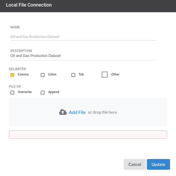
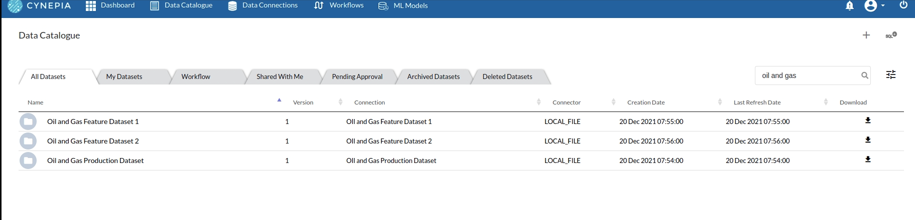
• Create a dataset for each dataset from the uploaded datasource in the data catalogue. Refer to Data Catalogue for more information on how to generate a dataset.

Create the Workflow for the experiment

• Lets Create our Workflow by going to the Workflows Tab in the Navigation. Create Workflow) has more information on how to create a workflow.

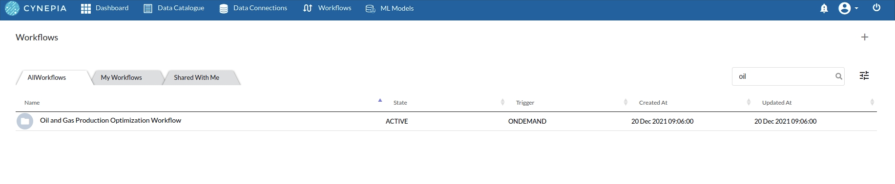
• We'll see an entry on the workflow's page listing our workflow once it's been created.

• To navigate to the workflow Details Page, double-click on the Workflow List Item and then click Design Workflow. Visit the Workflow Designer Main Page for additional information.
• By clicking on '+,' you can add the Input Dataset to the step view. The input step will be added to the Step View.

Perform initial exploration of data columns.

• Examine the output view with Header Profile, paying special attention to the column datatypes. Refer to Output Window for more information about the output window.

• Column Statistics Tab (Refer to Column Statisticsfor more details on individual KPI)

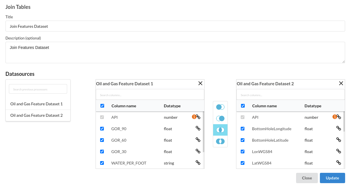
Perform Cleanup and Transform Operations

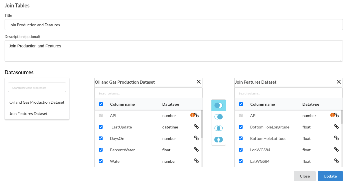
1. First Join the two features dataset . The processor used for this step is join tables

2. Join the features data with the production data . The processor used for this step is join tables

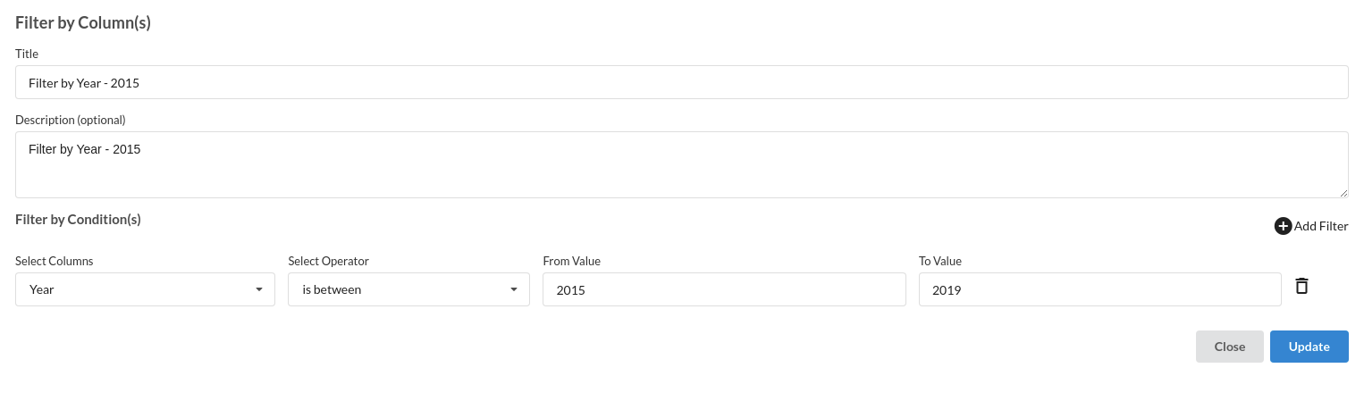
3. Filter by Year . The processor used for this step is filter records

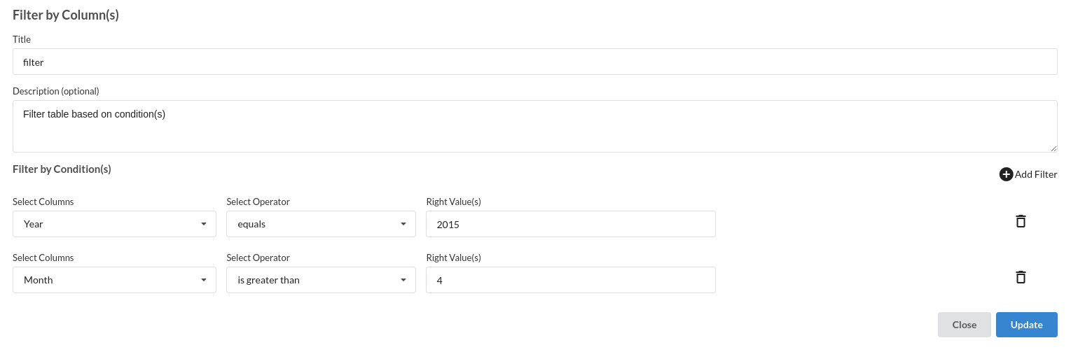
4. Filter Month. The processor used for this step is filter records

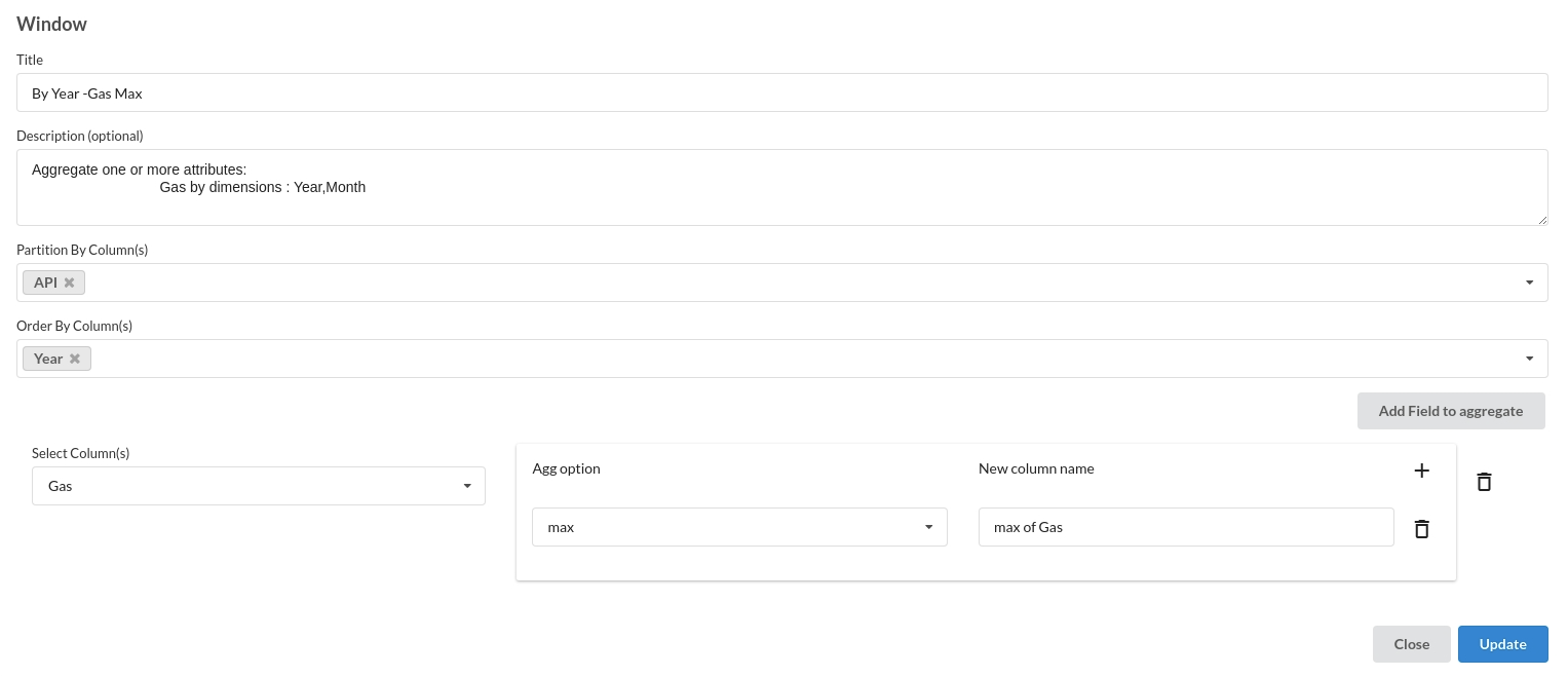
5. Window operation. The processor used for this step is Window

Build/Train a regression Model

• You now have a dataset to work with in order to create a regression model. Some of the actions to take before developing a model are listed below.

1. Feature Selection
2. Feature Encoding
3. Choose the algorithm and train the model.

Feature Selection

1. Go to the Column Profile View and select Multi-variate profile to construct a correlation matrix to manually identify the features of interest. The peason correlation is shown by Xceed Analytics. Select all of the columns that are strongly correlating to the target feature.

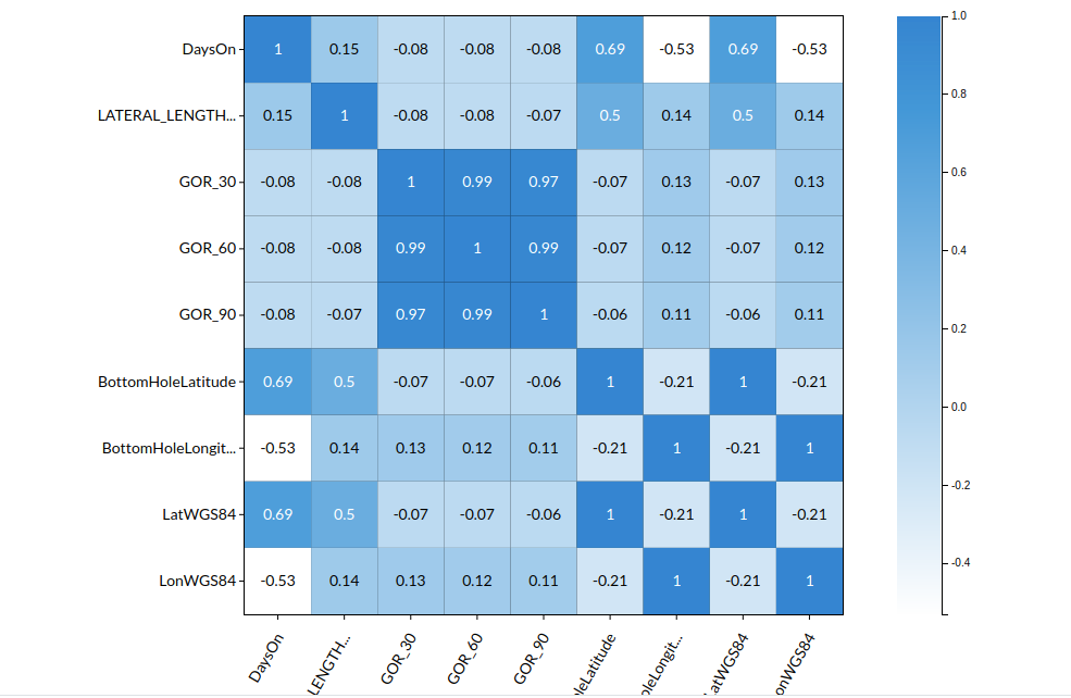
2. Some of the features we chose that can explain our target variable based on the observed correlation are:

• GOR 30
• GOR 60
• GOR 90
• DaysOn
• lat
• long etc

Feature Encoding

• Since all the features are already in the correct form and we dont have any categorical features, we omit this step for this workflow. for more information on this processor,refer to Feature encoding

Choose the algorithm and train the model.

• Because we're estimating a continuous variable- production  for the prediction model. From the Transformer View, select Regression(auto pilot) and put in the relevant information. Refer to Regression (autopilot)for more information on model parameters (autopilot)

Review the model output and Evaluate the model

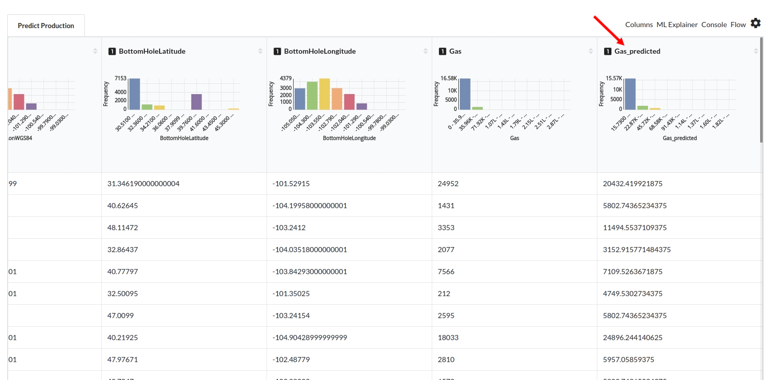
After you finish building the model, it is time to review the model output. Look at the output window to first review your predicted results .Since this is a regression problem you will get a new column in the view like the one below.

When you finish building your model you will see another tab in the view called Ml explainer . Click on that to evaluate your model.

• The first view you see when you click on ML explainer is the Summary view

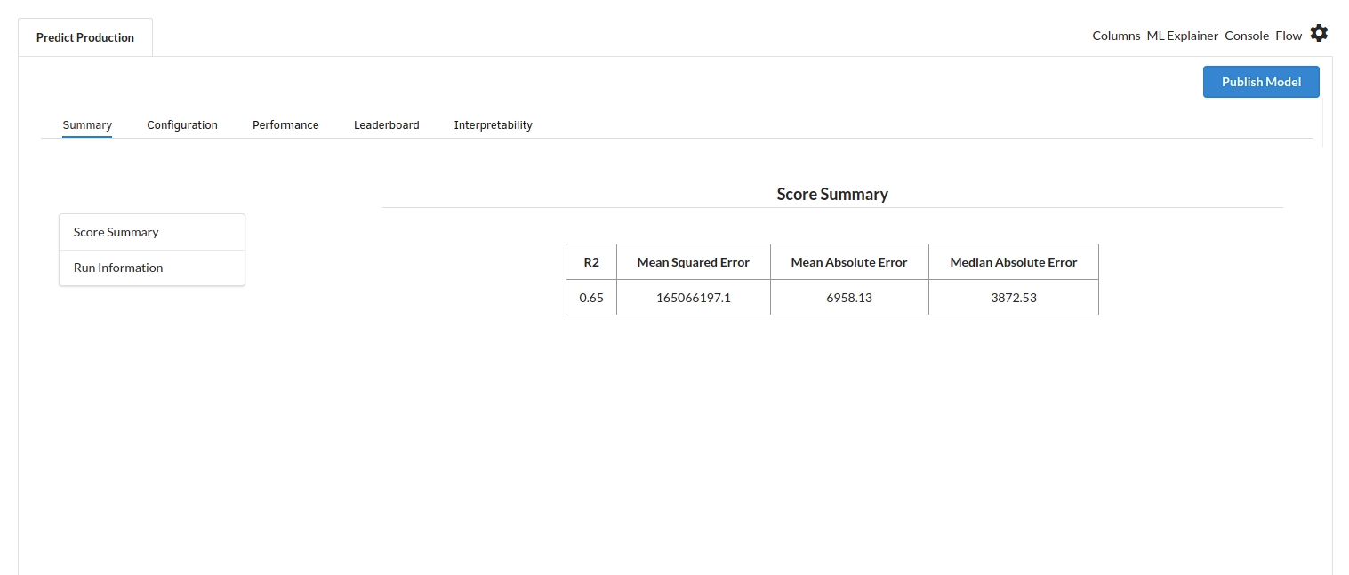
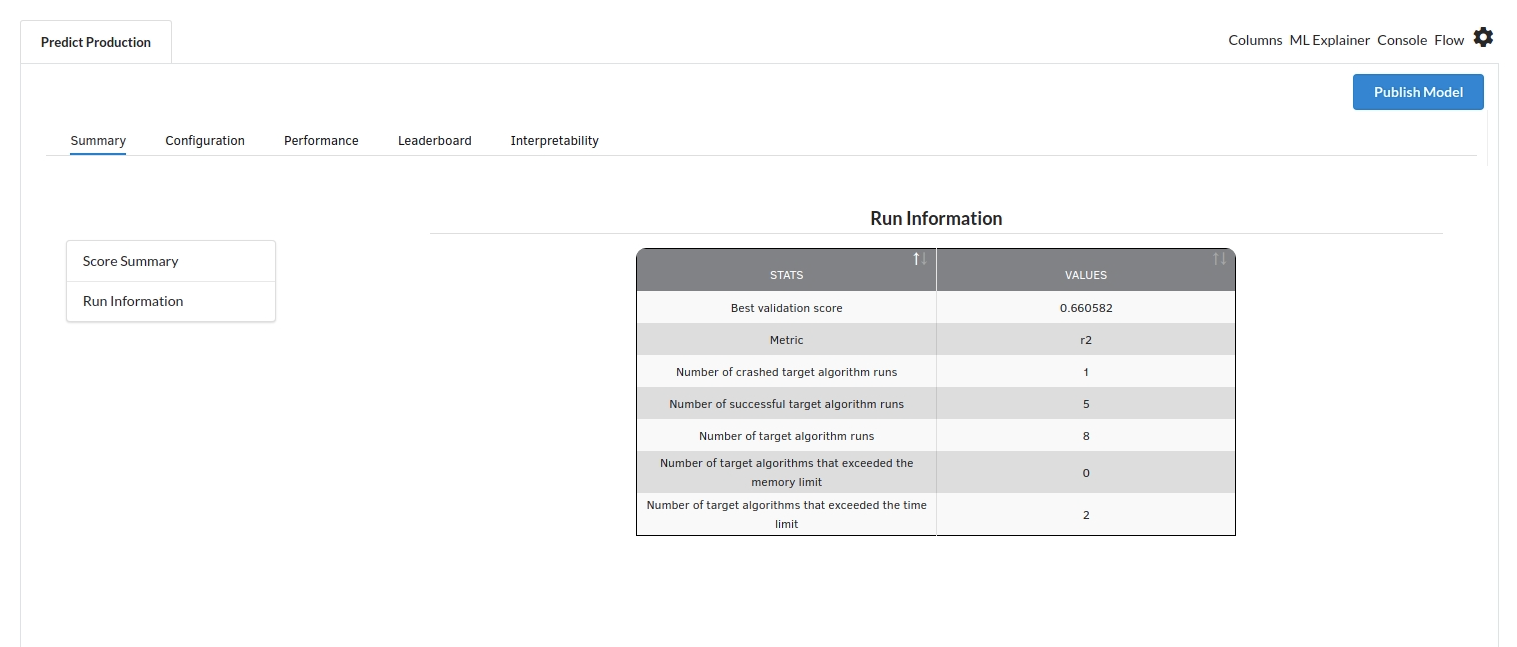
Look at the metrics score and the Run summary stats. Based on your calculations decide if the R2, mean Sqaured Error and Mean Absolute Error are according to your expecation. if not this will be your first step to rethink the training process.

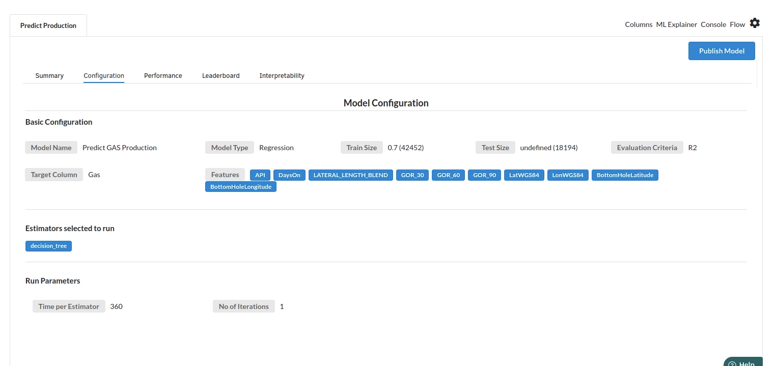
• The second view under Ml explainer is configuration view

The configuration view will give you the information about the step you filled in the Regression step . The view would look like the one below.

• The third view under Ml explainer is Performance View . You can see the actual vs predicted and the residual curve charts for regression. Look at the built charts and decide if the charts are good enough for your model. The actual vs predicted chart is a good indicator to understand how well your model was trained .

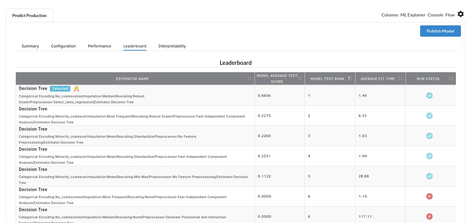
• The fourth view under Ml explainer is Leaderboard . In this view you can see the number of algorithms trained and all the feature engineering done on the algorithms used with ranking system to rank the best algorithm trained.

• The last view you see under ML explainer is Interpretability . In this view you will be able to interpret your model in simple terms where you will be getting results pertaining to feature importance , PDP Plots , Sub Population Analysis , Independant Explanation , Interactive Scoring . for more infomation on these results , refer to Interpretability . The Interpretability tab and the results under this tab would look like the one below.

1. Feature Importance

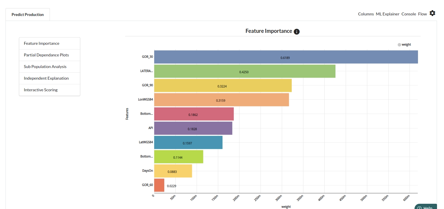
2. Partial Dependance Plots

3. Sub population analysis