Crop Yield Prediction Based on Climate Conditions

Background

Agriculture has been the oldest and prime activity through out the human history. However, over years a lot productivity benefits accrued in secondary and tertiary sectors and agriculture productivity in majority of countries remained stagnant. Hence, the contribution of agriculture to countries and their gdp kept shrinking over decades. Yet, It remains the most essential economic activity for human survival. It is also a crucial sector in the context of development countries such as India, since it still contributes to an outsized portion of employment.

World population continues to grow and is expected to peak at 11 billion by the year 2200 from the current approx 8 billion. Without increasing the farm prooductivity and planning at a country level, it would be challenging to produce enough food and ensure food security for a growing world population. There are also threats emerging in the form of climate change, which are leading to unpredented change in climate patterns that are further affecting farm production and creating unwanted losses for the farm businesses. In developing countries such as India, where share of irrigatable land as a percentage of total cultivatable land is only 35%, it is even more paramount to review the crop selection in context of the climate conditions. Therefore, helping farm businesses select appropriate crop is one of the important support need that central/state or district level agriculture institutes can help.

Crop yield is a standard measurement of the quantity of agricultural production harvested per unit of land area (i.e. yield of a crop ).

Objective

This usecase help predict production volume based on crop type, climate conditions, rainfall and various other geographical parameters. Output can be used by for various econometric and statistical planning.

Relevance of Xceed Analytics

Xceed Analytics provides a single integrated data and AI platform that reduces friction in bring data and building machine models rapidly. It further empowers everyone including Citizen Data Engineers/Scientist to bring data together and build and delivery data and ml usecases rapidly. It's Low code/No code visual designer and model builder can be leveraged to bridge the gap and expand the availability of key data science and engineering skills.

This usecase showcases how to create, train/test, and deploy a crop yield production regression model. The datasets are obtained from UCI. Crop datasets, rainfall datasets, and temperature datasets are among them.Starting with the uploading of datasets from multiple sources through the deployment of the model at the end point,

As mentioned earlier, we will use NO-CODE environment for the end-to-end implementation of this project. All of these steps are built using Visual Workflow Designer, from analyzing the data to constructing a model and deploying it.

Data Requirements

the following datasets are used for this usecase.

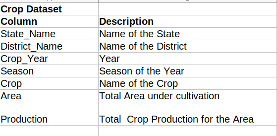
1. crop dataset : contains information on crops and their production by area, season, year, and location (State and District)
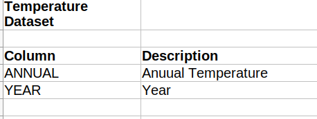
2. rainfall dataset : contains the annual rainfall information by year and location
3. temperature dataset: contains information about annual temperature by year

Available Features:

Crop Dataset:

Rainfall Dataset:

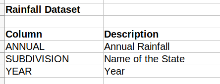
Temperature Dataset:

Model Objective

Understanding the trends of crop yield and estimating crop production by analyzing the underlying data and constructing a regression ML model and deploying it after understanding what were the significant features from the model is the outcome expected from this approach.

Steps followed to develop and deploy the model

1. Upload the data to Xceed Analytics and create a dataset
2. Create the Workflow for the experiment
3. Perform initial exploration of data columns.
4. Perform Cleanup and Tranform operations
5. Build/Train a regression Model
6. Review the model output and Evaluate the model

Upload the data to Xceed Analytics and Create the dataset

• From the Data Connections Page, upload the three datasets to Xceed Analytics: crop, rainfall, and temperature. For more information on Data Connections refer to Data Connectors

• Create a dataset for each dataset from the uploaded datasource in the data catalogue. Refer to Data Catalogue for more information on how to generate a dataset.

Create the Workflow for the experiment

• Creata a Workflow by going to the Workflows Tab in the Navigation. Create Workflow has more information on how to create a workflow.

• you will see an entry on the workflow's page listing our workflow once it's been created.

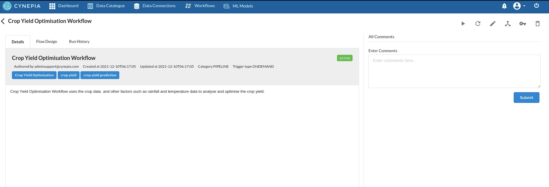
• To navigate to the workflow Details Page, double-click on the Workflow List Item and then click Design Workflow. Visit the Workflow Designer Main Page for additional information.
• By clicking on + icon you can add the Input Dataset to the step view. The input step will be added to the Step View.

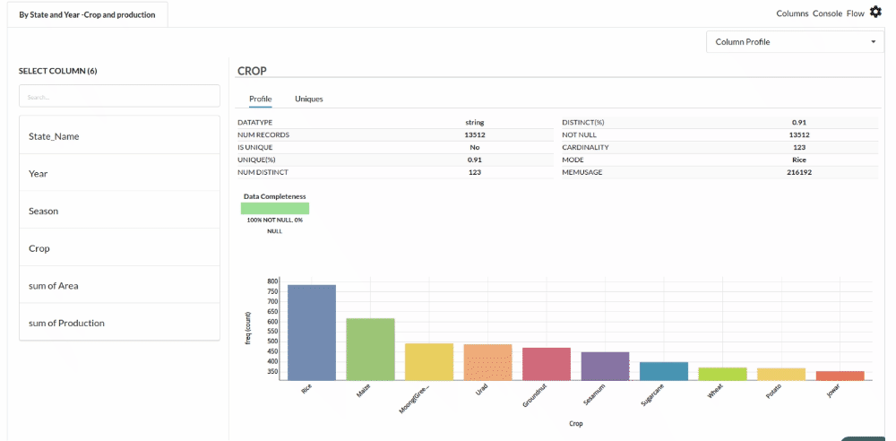
Perform initial exploration of data columns.

• Examine the output view with Header Profile, paying special attention to the column datatypes. Refer to Output Window for more information about the output window.

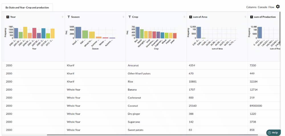
• Column Statistics Tab (Refer to Column Statisticsfor more details on individual KPI)

Perform Cleanup and Transform Operations

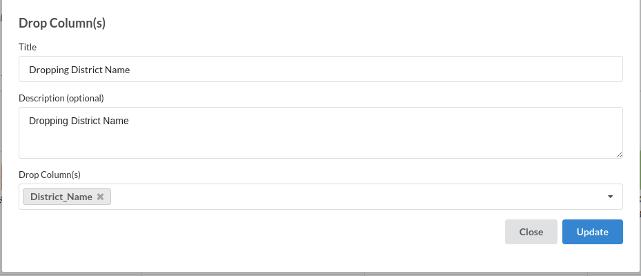
• Before we can build our model, we need to perform a few cleanup modifications.

1.Dropping irrelevant columns. The processor used for this step is Drop columns

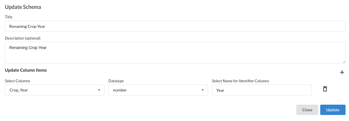
2.Rename Column. The processor used for this step is Update Schema

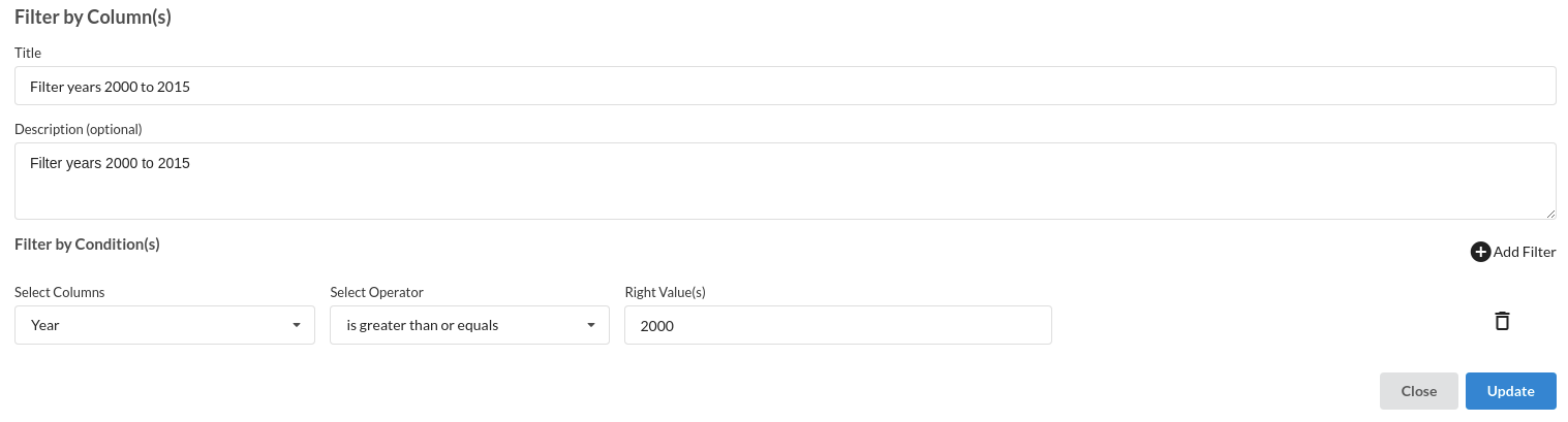
3.Filter by Year . The processor used for this step is filter records

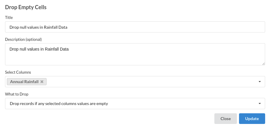
4.Drop Null values . The processor used for this step is drop empty cells

Build/Train a regression Model

• You now have a dataset to work with in order to create our regression model. Some of the actions we take before developing a model are listed below.

1. Feature Selection 2 .Feature Encoding
2. Choose the algorithm and train the model.

Feature Selection

1. Go to the Column Profile View and select Multi-variate profile to construct a correlation matrix to manually identify the features of interest. The peason correlation is shown by Xceed Analytics. Select all of the columns that are strongly correlating to the target feature.

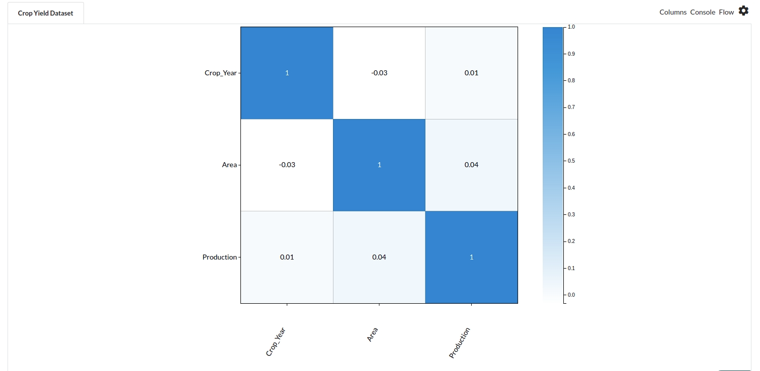
2. Some of the features to choose that can explain our target variable based on the observed correlation are:
   • Sum of Area
   • Annual Rainfall
   • Season etc.

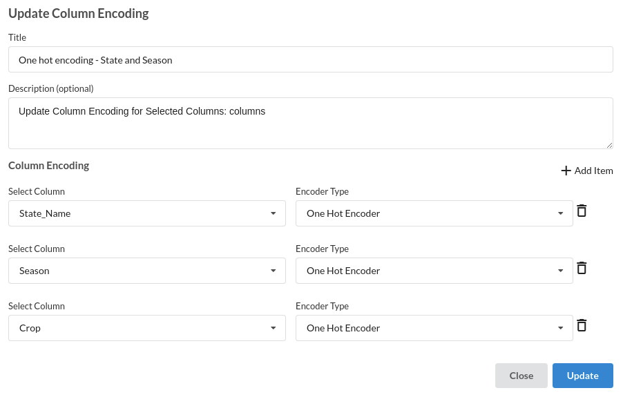
Feature Encoding

• Take all of the categorical columns and encode them based on the frequency with which they occur. The processor used for this step is Feature encoding

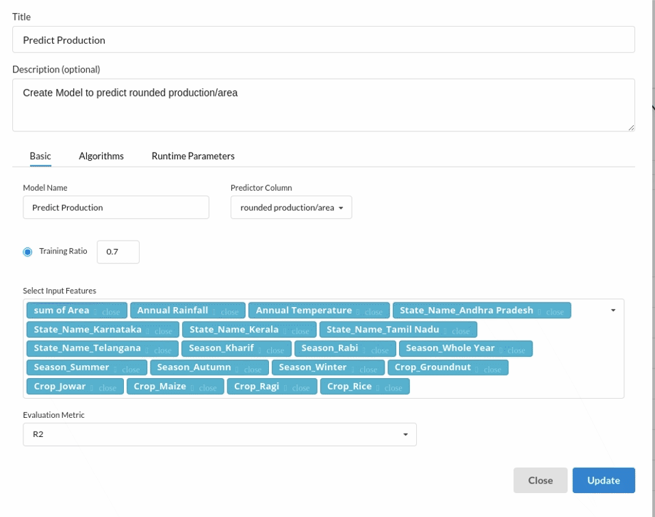
.Choose the algorithm and train the model.

• Because we're estimating a continuous variable- production  for the prediction model. From the Transformer View, select Regression(auto pilot) and put in the relevant information. Refer to Regression(auto pilot) for more information on model parameters (autopilot)

Review the model output and Evaluate the model

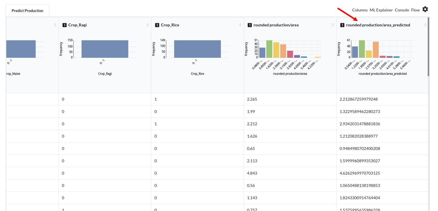
After you finish building the model, it is time to review the model output. Look at the output window to first review your predicted results .Since this is a regression problem you will get a new column in the view like the one below.

When you finish building your model you will see another tab in the view called Ml explainer . Click on that to evaluate your model.

• The first view you see when you click on ML explainer is the Summary view

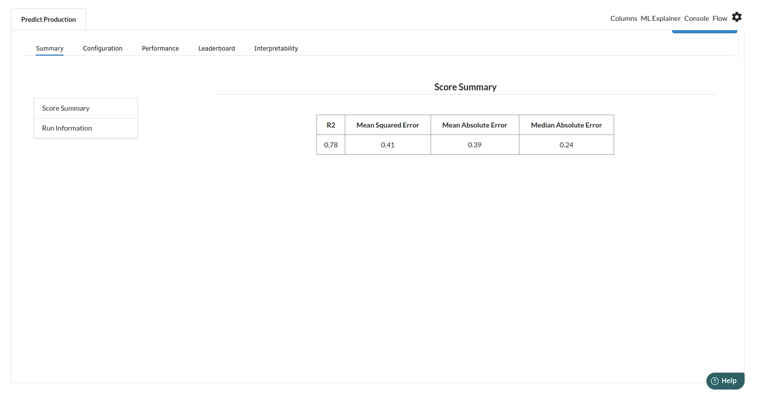
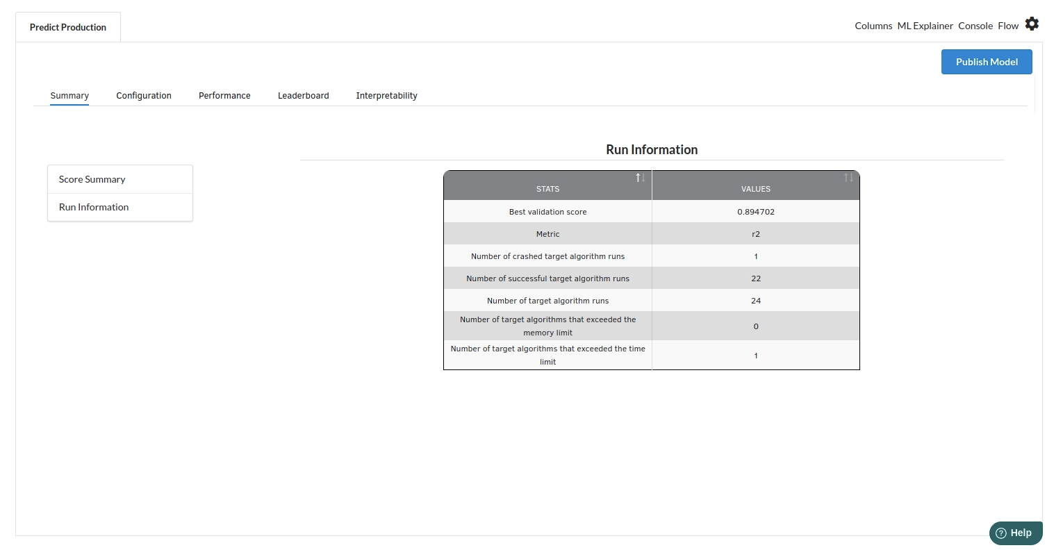
Look at the metrics score and the Run summary stats. Based on your calculations decide if the R2, mean Sqaured Error and Mean Absolute Error are according to your expecation. if not this will be your first step to rethink the training process.

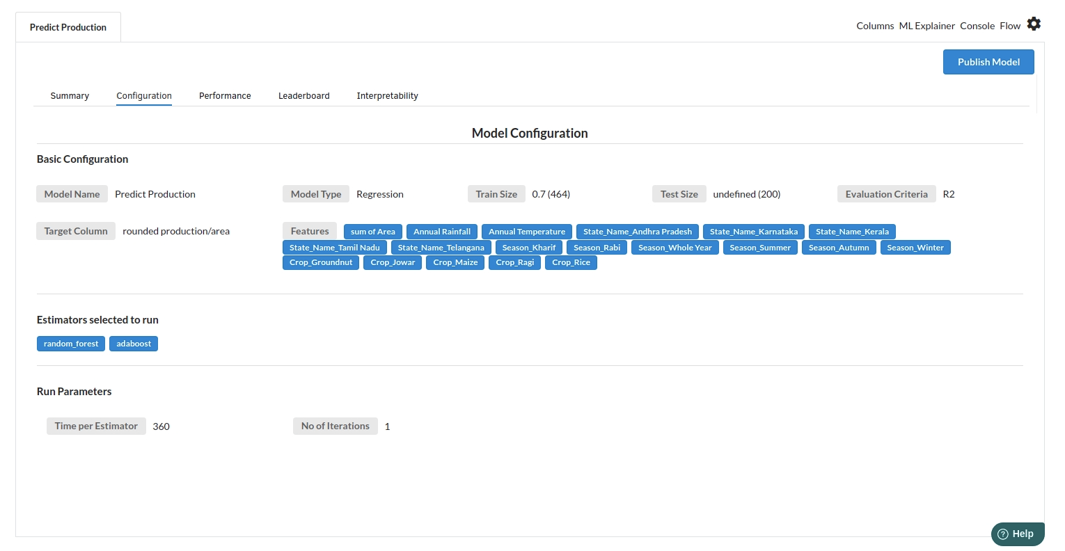
• The second view under Ml explainer is configuration view

The configuration view will give you the information about the step you filled in the Regression step . The view would look like the one below.

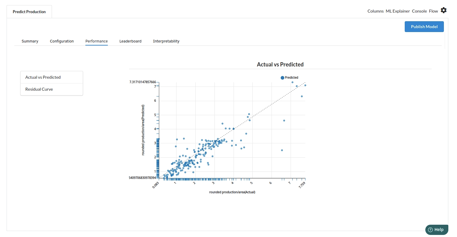
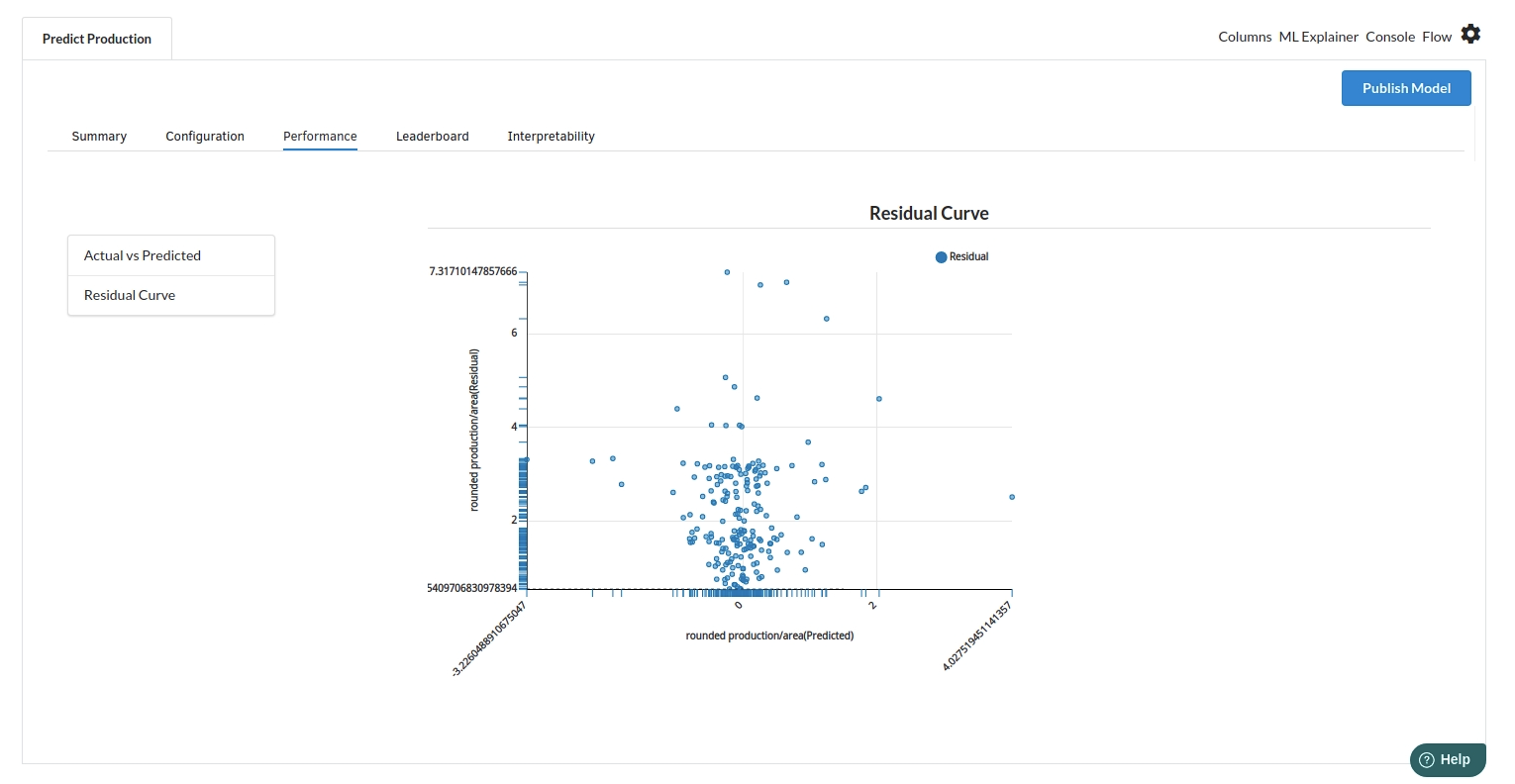
• The third view under Ml explainer is Performance View . You can see the actual vs predicted and the residual curve charts for regression. Look at the built charts and decide if the charts are good enough for your model. The actual vs predicted chart is a good indicator to understand how well your model was trained .

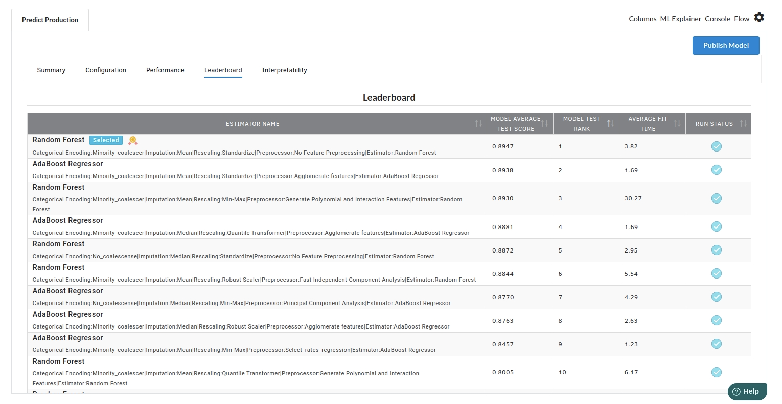
• The fourth view under Ml explainer is Leaderboard . In this view you can see the number of algorithms trained and all the feature engineering done on the algorithms used with ranking system to rank the best algorithm trained.

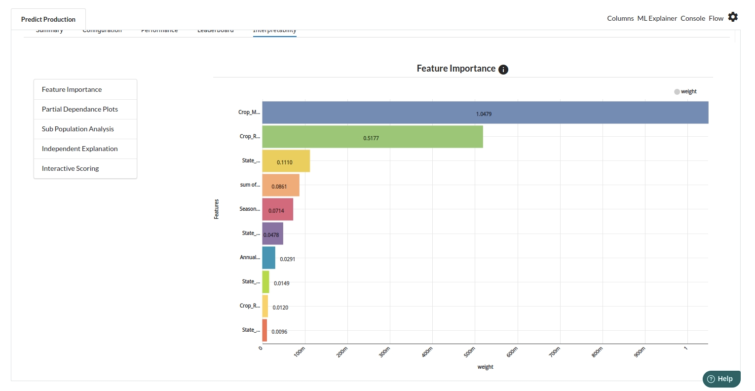
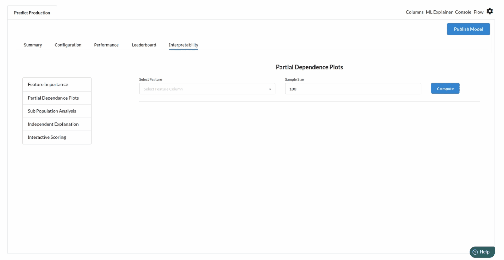
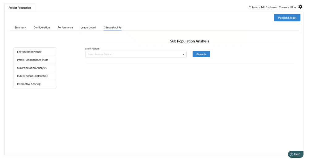
• The last view you see under ML explainer is Interpretability . In this view you will be able to interpret your model in simple terms where you will be getting results pertaining to feature importance , PDP Plots , Sub Population Analysis , Independant Explanation , Interactive Scoring . for more infomation on these results , refer to Interpretability . The Interpretability tab and the results under this tab would look like the one below.

Conclusion