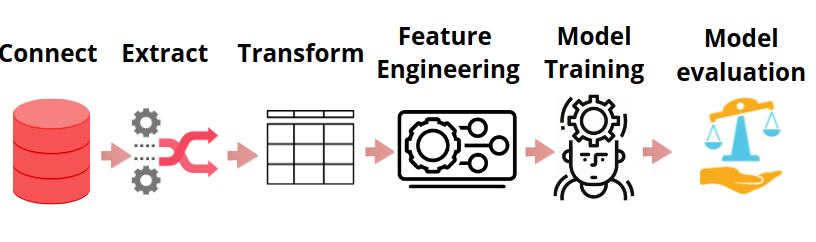
Model Building

Creating the Project

There are few steps to be followed before any model building is done:

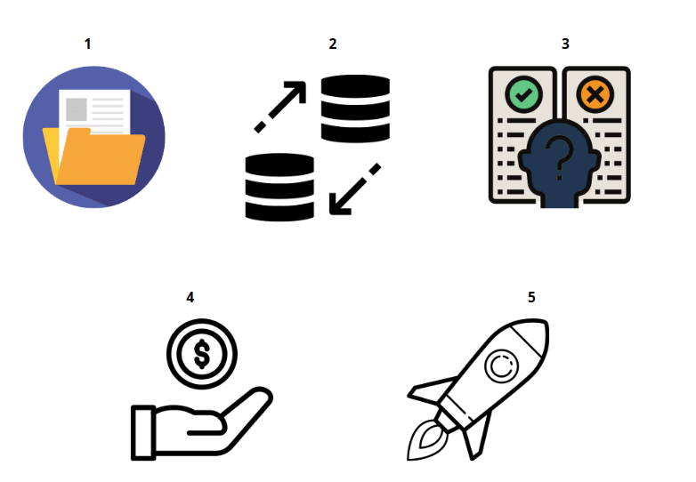
1. Build a proper use case. Understand if you want to solve Classification or Regression
2. Decide if you have proper data requrired for the usecase.
3. Define your hypothesis
4. Define what should be the outcome and what value would it give you or the organisation
5. Decide where and how will you deploy it .

Data Exploration

The primary goal of EDA is to maximize your insight into a data set and into the underlying structure of a data set, while providing all of the specific items that you would want to extract from a data set, such as:

1. A list of outliers
2. Conclusions as to whether individuall factors are statistically important/significant.
3. To understand the data in a much better way.
4. To test your hypothesis It is a good practice to understand the data first and try to gather as many insights from it. EDA is all about making sense of data in hand,before getting them dirty with it.

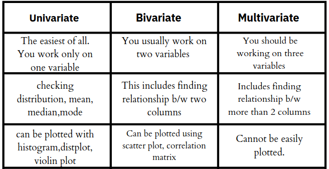
There are three kinds of analysis to be done when you start exploring any data:

1. Univariate analysis : this is the simplest of the three analyses where the data you are analyzing is only one variable. There are many different ways people use univariate analysis. The most common univariate analysis is checking the central tendency (mean, median and mode), the range, the maximum and minimum values, and standard deviation of a variable.
2. Bivariate Analysis : Bivariate analysis is where you are comparing two variables to study their relationships. These variables could be dependent or independent to each other. In Bivariate analysis is that there is always a Y-value for each X-value.The most common visual technique for bivariate analysis is a scatter plot, where one variable is on the x-axis and the other on the y-axis.
3. Multivariate Analysis : Multivariate analysis is similar to Bivariate analysis but you are comparing more than two variables. For three variables, you can create a 3-D model to study the relationship (also known as Trivariate Analysis).

Cleaning Datasets & Feature Engineering

Cleaning Datasets and Feature Engineering involves in the understanding, formatting , transforming and selecting the features to train a machine learning model.

There are 4 parts of Feature Handling:

1. Feature Representation
2. Feature Selection
3. Feature Transformation
4. Feature Engineering

Feature Representation

To showcase your data to any algorithm , your data needs to represented as quantitative attributes(preferably numeric). Often in real world data you will come across textual data and luckily there are few techniques that can change your textual data into numerical . few of them are :

1. One Hot Encoder : Representation of categorical variables into binary vectors. If you have a column named category and it has around 3 categories such as clothing,furniture, appliances, then you One Hot Encoder will turn them into three different columns and create binary values wherever these values occur in the dataset.
2. Label Encoder : In this each label or row value in a column is assigned a unique integer based on alphabetical ordering. This can be a manual process too based on your requirement.

Feature Selection

In machine learning or statistics ,Feature selection is also known as variable selection , attribute selection . Feature selection is a process of reducing the number of input variables when developing a predictive model. Reasons why Feature selection is important is:

• Simplification of models for human interpretability.
• Shorther training time or less compute
• To avoid the curse of dimensionality: In simple terms it means, The error increases with increase in number of features.

There are some techniques to Feature Selection:

1. Filter Methods : these are methods where you automatically or manually select features by looking at the correlational matrix.
2. Wrapper Methods: One of the examples under this method is called RFE (Recursive feature elimination). RFE can be used for both classification an regression models.

Refer Feature Selection techinques for more information on this topic

Feature Engineering

The process of cleaning your dataset can be termed as Feature Engineering.In other words, Feature Engineering is turning raw data into useful data so that all the ML algorithms will be able to ingest them properly. The first and foremost necessity is to decide whether your data needs cleaning or not. for that you need to explore your data which is also known as EDA(Exploratory Data Analysis). after that you can perform feature engineering.

The basic steps one should follow under Feature Transformation are :

1. check for the datatypes of the columns and change them accordingly. suppose age of a person is a categorical column then it should be changed to numerical column.
2. If your dataset contains null values then you need to fill them or empty the rows where you have null values.

• Median
• Mode
• backword fill
• forward fill

3. Check if your dataset contains duplicates and evaluate if they are actually duplicates. After thorough assessment you can choose to drop them.
4. Check for Outliers in your data and decide if they are actually outliers and then filter them out. One of the ways to do that is to plot a box plot or a scatter plot .
5. See the distribution of the data, see the skewness and kurtosis of all the columns. You can plot histogram to see for the distribution of the data.
6. Handle Imbalance of the data. This is something every datascience professional needs to understand. Handling Imbalance of the data means getting good and equal samples of your data. For example, take a column age and when you do EDA you find out that the age of 20-30 values are way more than the ones in the other age bracket then your job should be to sample the dataset where youget equal number of instance to get all age brackets in one set.

Few of the techniques for handling Imbalance of the data are :

1. Sample your dataset: there are two ways to sample a dataset:

• Under Sampling: Under-sampling balances the dataset by reducing the size of the abundant class. This method is used when quantity of data is sufficient.
• Over Sampling : oversampling is used when the quantity of data is insufficient. It tries to balance dataset by increasing the size of rare samples.
• Cluster based Over Sampling: K-means clustering algorithm is independently applied to minority and majority class instances. This is to identify clusters in the dataset.

Feature Transformation

Just as oil needs to be refined before it is used, similarly data needs to be refined before we use it for machine learning. In most of the usecases you work on you may have to derive new features out of existing features. This can also be a part of Feature Engineering but if we go the shape and complexity then calling this as feature transformation makes sense.

Below are some of the few Feature Transformation techniques:

1. Aggregation : New features are created by getting a count, sum, average, mean, or median from a group of entities.
2. Part-Of : New features are created by extracting a part of data-structure. E.g. Extracting the month from a date.
3. Binning — Here you group your entities into bins and then you apply those aggregations over those bins. Example — group customers by age and then calculating average purchases within each group.
4. Flagging :Here you derive a boolean (0/1 or True/False) value for each entity

Creating the Model

This is the final part of the model building process where you will be selecting the columns required , splitting the dataset into different sets, Choosing the algorithm and train it . Steps included under Creating a model are :

1. Feature Selection
2. Splitting the data
3. Choose an algorithm
4. Choose the evaluation metric
5. Hyperparameter Tuning
6. Training the Algorithm

Select the Features

After you finish cleaning and feature engineering the data you need to decide what all columns to select to build a model, this process can be done using many methods such as :

1. Filter Methods
2. Fisher's score
3. Correlation matrix

But, the most effective and widely used method is Correlation matrix .

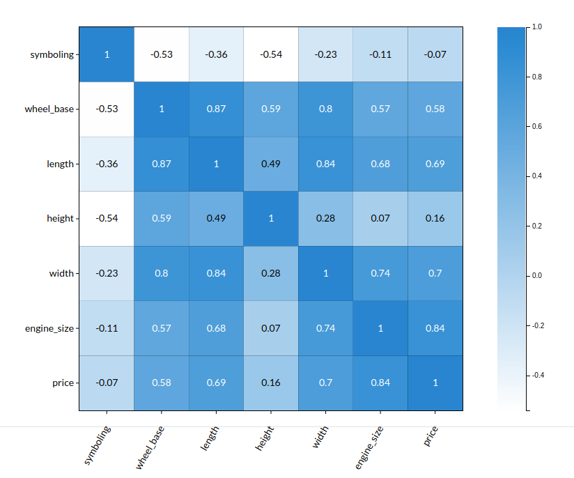
A correlation matrix is simply a table which displays the correlation coefficients for different variables. The matrix depicts the correlation between all the possible pairs of values in a table. It is a powerful tool to summarize a large dataset and to identify and visualize patterns in the given data.

You can read a correlational matrix easily by just comparing the predictor column with an independant column.

note

• Predictor column is the column which is to be predicted after training the model. suppose price is the predictor column then price is the column which needs to be predicted after model building.
• Independant columns are the columns which are apart from the predictor column because based on the Independant columns the prediction happens.

Take the example from above . You can see a column called price . let us consider that to be our predictor column and the other columns as our independant columns.

• take the predictor column and choose a column of your choice and check for their correlation.
• Higher the number or darker the shade of the block, the higher the correlation.
• You can also negative numbers when compared with the price , those are nor correlating with the predictor so it is best to not take that column when you train your model.

for more information, refer to feature selection

Test vs Train Split

The train-test split procedure is used to estimate the performance of machine learning algorithms when they are used to make predictions on data not used to train the model. This is a very easy process but one needs to be careful as to what should be the configuration for training and testing the data and also Train-Test split makes sense when you have a large dataset .

The procedure involves taking a dataset and dividing it into two subsets. The first subset is used to fit the model and is referred to as the training dataset. The second subset is not used to train the model; instead, the input element of the dataset is provided to the model, then predictions are made and compared to the expected values. This second dataset is referred to as the test dataset.

• Train Dataset: Used to fit the machine learning model.
• Test Dataset: Used to evaluate the fit machine learning mode.

You must choose a split percentage that meets your project’s objectives with considerations that include:

• Computational cost in training the model.
• Computational cost in evaluating the model.
• Training set representativeness.
• Test set representativeness.

The most common Train-Test split percentage are :

• Train: 80%, Test: 20%
• Train: 67%, Test: 33%
• Train: 50%, Test: 50%

As an example see how Xceed does the train test split in a classsification model

Select the Estimators/Algorithms to run

Having a wealth of options is good, but deciding on which model to implement in production is crucial. Though we have a number of performance metrics to evaluate a model, it’s not wise to implement every algorithm for every problem. This requires a lot of time and a lot of work. So it’s important to know how to select the right algorithm for a particular task.

Choose the Evaluation Metric

In order to test a model, an appropriate evaluation metric must be chosen during the model development, which is subsequently used as a measure to evaluate the model performance against the test data, during production as well as over time when different revisions of the model are built. Besides, each of the available metric type must associate with the given business use case.

For example, In case of Binary Classification problem such as a Loan Default or Spam Detection, Given the actual data may be imbalanced in favour of non-defaulters, Accuracy is a poor metric to select, since Accuracy reflects the overall model performance and may not give the insights on how well it performed on the minority class (which in this case is default cases). Likewise in case of regression use cases, if a few outlier max values are acceptable MAE may be an exceptable metric, However, in cases where we care for Maximum Error, RMSE may be a far more balanced metric to choose.

As an example see what all criterias does Xceed Support under ML explainer Tab

Factors that matter the most when choosing a machine learning algorithm:

1. Interpretability:When you think about the interpretability of an algorithm, You should understand its power to explain its predictions. An algorithm that lacks in such an explanation is called a black-box algorithm. Algorithms like the k-nearest neighbor (KNN) have high interpretability through feature importance. And algorithms like linear models have interpretability through the weights given to the features. Knowing how interpretable an algorithm becomes important when thinking about what your machine learning model will ultimately do.

2. The Size of the dataset:When selecting a model, the size of the dataset and the number of features play a vital role, In some cases, the selection of the algorithm comes down to understanding how the model handles different sizes of datasets.

3. Linearity of the data :Understanding the linearity of data is a necessary step prior to model selection. Identifying the linearity of data helps to determine the shape of the decision boundary or regression line, which in turn directs us to the models we can use. Some relationships like height-weight can be represented by a linear function which means as one increases, the other usually increases with the same value. Such relationships can be represented using a linear model.

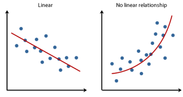
If the data is almost linearly separable or if it can be represented using a linear model, algorithms like SVM, linear regression, or logistic regression are a good choice.

4. Training Time :Training time is the time taken by an algorithm to learn and create a model. For use cases like movie recommendations to a particular user, data needs to be trained every time the user logs in. But for use cases like stock prediction, the model needs to be trained every second. So considering the time taken to train the model is essential.

5. Memory Requirements :If your entire dataset can be loaded into the RAM of your server or computer, you can apply a vast number of algorithms. However, when this is not possible you may need to adopt incremental learning algorithms. Incremental learning is a method of machine learning where input data is continuously used to extend the existing model’s knowledge, i.e. to train the model further.

6. Prediction Time : Prediction time is the time it takes for the model to make its predictions. For internet companies, whose products are often search engines or online retail stores, fast prediction times are the key to smooth user experience. In these cases, because speed is so important, even an algorithm with good results isn’t useful if it is too slow at making predictions. However, it’s worth noting that there are business requirements where accuracy is more important than prediction time. This is true in cases such as the cancerous cell example we raised earlier, or when detecting fraudulent transactions.

Hyperparameter Tuning

Hyperparameters are high level attributes that are supposed to set before the model is assembled.For example, if you are building model using random forest algorithm where decision trees will be split but the number of splits should be determined by you before hand. So, In short your hyperparmeters are the variables that govern the training process itself. Two of the most efficient methods to find best hyperparameters for any model are :

1. Grid Search Cv : GridSearchCV is a library function that is a member of sklearn’s model_selection package. It helps to loop through predefined hyperparameters and fit your estimator (model) on your training set. So, in the end, you can select the best parameters from the listed hyperparameters.

2. Randomised Search CV : RandomizedSearchCV solves the drawbacks of GridSearchCV, as it goes through only a fixed number of hyperparameter settings. It moves within the grid in random fashion to find the best set hyperparameters. This approach reduces unnecessary computation.

for more information , refer to Hyperparameter Tuning

Train