Model Evaluation

Model Evaluation is an important step in understanding the correctness of model on the test data. As you already are aware, test data deals which the set of data points not seen by the model prior. Once we get the predictions on the test data, we compare the same with the actual values of the predictor variable. There are a wide range of metrics, that can help understand/evaluate how well did the model perform with the test data.

Metrics are measures of quantitative assessment commonly used for comparing, and tracking performance of any system/process

Why do you evaluate the model

Model Evaluation process is key to understanding if the model successfully learnt the business parameters fed and meets the business objectives laid out for the project effectively. Following are some of the important answers to look out for:

1. Is the model good at predicting the target on new and future data (which may be unknown) ?
2. Is it good to deploy it into production ?
3. will a larger training set improve the model's performance
4. Does the model have high bias and is oversimplifying the actual problem statement, by ignoring majority of data points in the training set and deriving the answers on a few fields and data points ? (Also called Underfitted)
5. Does the model have high variance ? A model with high variance will restrict itself to the training data and will not be great at predicting on unseen data or future data. Essentially, by not generalizing the rules and trying to answer based on specific data learning (Often termed as Overfitted Models)
6. Do we need to source more training data, add/remove features, source/select different algorithm or even different metric to meet the project objective?
7. If one is concerned about bias, One may also want to evaluate model performance across various population sub-groups.

In summary, Model Evaluation Metrics help you perform test of fitness of model for future use. There are a wide range of metrics that can be put to use. Broadly these metrics are based on class of problem being solved.

Classification Related Metrics

After training a classification model there are 4 types of outcomes that could occur:

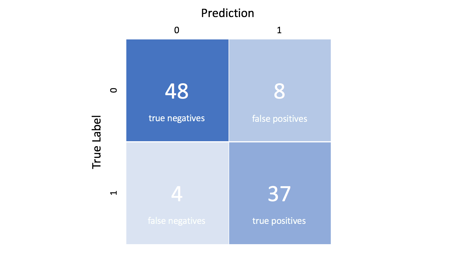
• True positive :True Positives are when you predict an observation belong to a class and it actually does belong to a class.
• True Negative : True negatives are when you predict an observation does not belong to a class and it actually does not belong to a class.
• False Positive : False Postives occur when you predict an observation belongs to a class when in reality it does not .
• False Negative : False Negative occur when you predict an observation does not belong to a class when in fact it does.

Confusion Matrix

A Confusion Matrix is an NxN matrix, where N is the number of classes being predicted. For Binary Classification Problems: N=2 and hence matrix will be 2x2 matrix.

These four outcomes are often plotted in a confusion matrix:

There are few other simpler metrics to measure the performance of a classification model

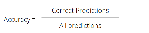
1. Accuracy : Accuracy is defined as the percentage of correct predictions for the test data. Essentially, it looks at accuracy at overall test data level. It is calculated by dividing number of correct predictions by the total number of predictions as shown below:

You need to decide whether accuracy is be-all and end-all metric that shall choose your model's best form.

Look at the below confusion matrix

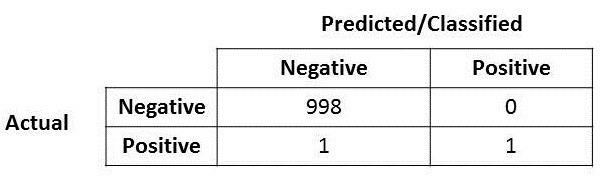
Looking at the actual vs predicted you may have guessed your model's accuracy is 99.9%. While most of us can be happy if that were the case but 99.9% can be a very dangerous number for any organisation.what if the positive over here is actually someone who is sick and carrying a virus that can spread very quickly? Or the positive here represent a fraud case?. The cost of having mis-classified actual positive is very high in these scenarios. So, the conclusion is accuracy is not the only metric you need for your model.

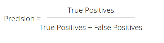
2. Precision: Precision is defined as the fraction of relevant examples (true positives) among all of the examples which were predicted to belong in a certain class. The formula to calculate precision is shown below:

In simple words this formula explains True Positive / Total Predicted Positive (Including ones wrongly predicted as Positive)

Precision is a good measure to determine, when the costs of False Positive is high. For instance, email spam detection. In email spam detection, a false positive means that an email that is non-spam (actual negative) has been identified as spam (predicted spam). The email user might lose important emails if the precision is not high for the spam detection model.

3. Recall: Recall is defined as the fraction of examples which were predicted to belong to a class with respect to all of the examples that truly belong in the class.The formula to calculate recall is shown below:

In simple words this formula explains True Positive / Total Actual Positive (Including ones wrongly predicted as Negative)

So, Recall actually calculates how many of the Actual Positives the model captured through labeling it as Positive (True Positive). Applying the same understanding, Recall shall be the model metric to use to select your best model when there is a high cost associated with False Negative.

For instance, in fraud detection or sick patient detection. If a fraudulent transaction (Actual Positive) is predicted as non-fraudulent (Predicted Negative), the consequence can be very bad for the financial institution.

4. F1 Score :

In previous two measures, we saw the importance of Precision and Recall and their relevance from specific use case point of view. Often there are use cases, where we need to get the best precision and best recall at the same time? F1-score is once such metric. It is essentially nothing but harmonic mean of precision and recall values. The formula to calculate F1 score is as below:

One may question, why does F1-score use harmonic mean and not an arithmetic mean. Harmonic mean punishes extreme values more. Let us understand this with an example. Lets say we have Precision is 0 and Recall is 1, In this case Arithmetic mean will be 0.5. A Harmonic mean on the other hand, will be 0, which is perfectly fine in the said example, since the model is of no use if it has precision as 0.

The harmonic mean is a type of numerical average. It is calculated by dividing the number of observations by the reciprocal of each number in the series. Thus, the harmonic mean is the reciprocal of the arithmetic mean of the reciprocals.

5. Log Loss : Log-loss is indicative of how close the prediction probability is to the corresponding actual/true value (0 or 1 in case of binary classification). The more the predicted probability diverges from the actual value, the higher is the log-loss value. Log Loss is the negative average of the log of corrected predicted probabilities for each instance

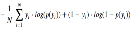
• Here Yi represents the actual class and log(p(yi)is the probability of that class.
• p(yi) is the probability of 1.
• 1-p(yi) is the probability of 0.

6. Area under the Curve - ROC-AUC: AUC - ROC curve is a performance measurement for the classification problems at various threshold settings. ROC is a probability curve and AUC represents the degree or measure of separability. It tells how much the model is capable of distinguishing between classes. Higher the AUC, the better the model is at predicting 0 classes as 0 and 1 classes as 1. By analogy, the Higher the AUC, the better the model is at distinguishing between patients with the disease and no disease.

An excellent model has AUC near to the 1 which means it has a good measure of separability. A poor model has an AUC near 0 which means it has the worst measure of separability. In fact, it means it is reciprocating the result. It is predicting 0s as 1s and 1s as 0s. And when AUC is 0.5, it means the model has no class separation capacity whatsoever.

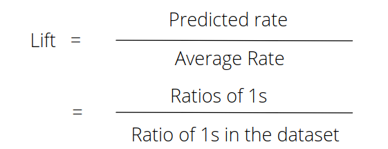
7. Lift Curves : lift is a measure of the performance of a targeting model (association rule) at predicting or classifying cases as having an enhanced response (with respect to the population as a whole), measured against a random choice targeting model.A lift curve shows the ratio of a model to a random guess ('model cumulative sum' / 'random guess The formula to calculate lift is :

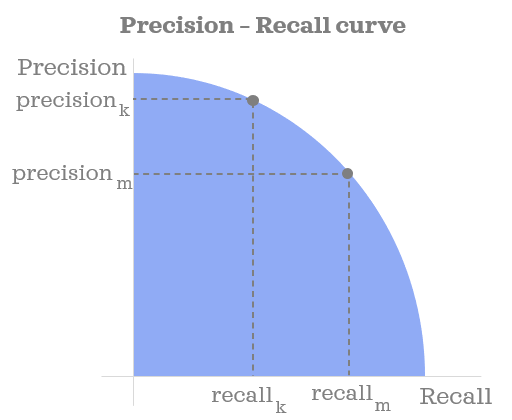
8. Precision Recall Curves : The precision-recall curve is used for evaluating the performance of binary classification algorithms. It is often used in situations where classes are heavily imbalanced. Also like ROC curves, precision-recall curves provide a graphical representation of a classifier’s performance across many thresholds, rather than a single value (e.g., accuracy, f-1 score, etc.). The precision-recall curve is constructed by calculating and plotting the precision against the recall for a single classifier at a variety of thresholds

Metrics for Regression

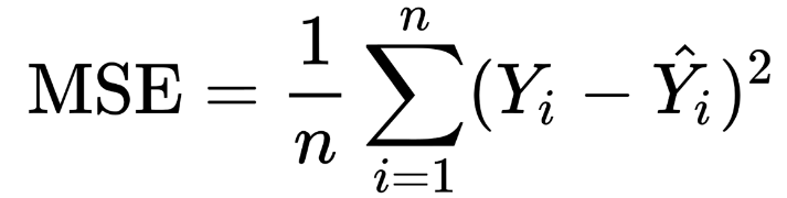
1. Mean Squared Error / Root Mean Squared Error : MSE is the average of the squared error that is used as the loss function for least squares regression.It is the sum, over all the data points, of the square of the difference between the predicted and actual target variables, divided by the number of data points. The formula to calculate Mean Squared Error is:

Root mean sqaured error is calculated by taking the root by MSE . the formula to calculate RMSE is :

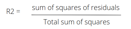
2. R-Squared: R-Squared is also known as the coefficient of determination. It works by measuring the amount of variance in the predictions explained by the dataset. it is the difference between the samples in the dataset and the predictions made by the model.If the value of the r squared score is 1, it means that the model is perfect and if its value is 0, it means that the model will perform badly on an unseen dataset. This also implies that the closer the value of the r squared score is to 1, the more perfectly the model is trained. The formula to calculate R-square is :

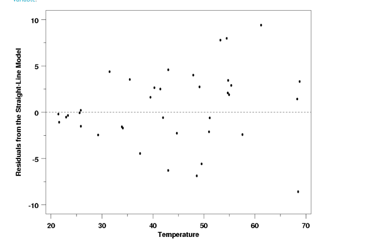
4. Residual Curve : A residual value is a measure of how much a regression line vertically misses a data point. Regression lines are the best fit of a set of data. You can think of the lines as averages; a few data points will fit the line and others will miss. A residual plot has the Residual Values on the vertical axis; the horizontal axis displays the independent variable.

A residual plot is typically used to find problems with regression. Some data sets are not good candidates for regression, including:

• Heteroscedastic data (points at widely varying distances from the line).
• Data that is non-linearly associated.
• Data sets with outliers.

5.Actual vs Target : Actual vs Target is a way to visualise the prediction done with the test data. The test data is plotted in the Y axis and the predicted values for the test data is plotted in the X axis. This is a feature given exclusively in Xceed- Workflow designer. It will help you understand how far off or how near are your predicted values.