Time Series Forecasting

What is Time Series data?

Time series is a collection of observations through repeated measurements over time. Time series data can also be referred to as time stamped data . These data points typically consist of successive measurements made from the same source over a time interval and are used to track change over time.In particular, a time series allows one to see what factors influence certain variables from period to period. Examples of Time Series Data :

1. Stock prices in any stock exchange.

2.ECG monitors.

3. Weather records.

What is Time Series analysis?

Time series analysis is a specific way of analyzing a sequence of data points collected over an interval of time. In time series analysis, analysts record data points at consistent intervals over a set period of time rather than just recording the data points intermittently or randomly. However, this type of analysis is not merely the act of collecting data over time. What sets time series data apart from other data is that the analysis can show how variables change over time. In other words, time is a crucial variable because it shows how the data adjusts over the course of the data points as well as the final results.

Where is time series analysis useful ?

Time series analysis is used for non-stationary data—things that are constantly fluctuating over time or are affected by time. Industries like finance, retail, and economics frequently use time series analysis because currency and sales are always changing. Stock market analysis is an excellent example of time series analysis in action, especially with automated trading algorithms. Likewise, time series analysis is ideal for forecasting weather changes, helping meteorologists predict everything from tomorrow’s weather report to future years of climate change. Because time series analysis includes many categories or variations of data, analysts sometimes must make complex models. However, analysts can’t account for all variances, and they can’t generalize a specific model to every sample. Models that are too complex or that try to do too many things can lead to lack of fit. Lack of fit or overfitting models lead to those models not distinguishing between random error and true relationships, leaving analysis skewed and forecasts incorrect.

What is time series forecasting?

Time series forecasting is the process of analyzing time series data using statistics and modeling to make predictions and inform strategic decision-making. It’s not always an exact prediction, and likelihood of forecasts can vary wildly—especially when dealing with the commonly fluctuating variables in time series data as well as factors outside our control. Series forecasting is often used in conjunction with time series analysis. Time series analysis involves developing models to gain an understanding of the data to understand the underlying causes. Analysis can provide the “why” behind the outcomes you are seeing. Forecasting then takes the next step of what to do with that knowledge and the predictable extrapolations of what might happen in the future.

When should you use Time series forecasting ?

Naturally, there are limitations when dealing with the unpredictable and the unknown. Time series forecasting isn’t infallible and isn’t appropriate or useful for all situations. Because there really is no explicit set of rules for when you should or should not use forecasting, it is up to analysts and data teams to know the limitations of analysis and what their models can support. Not every model will fit every data set or answer every question. Data teams should use time series forecasting when they understand the business question and have the appropriate data and forecasting capabilities to answer that question

Things to remember

• Time series can be irregulary placed : Typically the data will be collected in some interval such as by minutes, hourly,daily etc., But there are cases where the time series is irregular.
• Time series is mostly analysis : The main goal should not be to use a forecasting model . The problem space is in understanding if the data the organisations collect makes sense or all of that are just white noise.
• Should be careful with the missing values : Since Time series is a differnt space in Datascience and ML, it is not wise everytime to use techniques such as global mean or median for fill the empty values. Extreme exploration is required.

Types of time series forecasting models

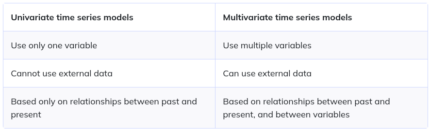
• Univariate Time series: Univariate time series deals with just one variable other than the date column . For example, data collected from a sensor measuring the temperature of a room every second. Therefore, each second, you will only have a one-dimensional value, which is the temperature.

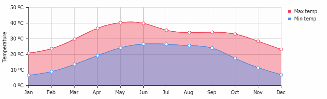
• Multivariate Time series : Multivariate time series deals with multiple variables other than the date column . For example , measuring the weather conditions based on date, temperature, season etc., is Multivariate time series.

Terminologies in Time series Forecasting

You will come across a lot of terms while doing time series analysis which are very important and useful . These terms are based on the premises of understanding the data.

• Time period : The interval of recording data from one date point to another date point is time period.

• Frequency : How often value of the dataset are recorded is called frequency . All time periods must be equal and clearly defined which would refult in a constant frequency.Most common frequency are hourly, daily , quarterly and yearly.

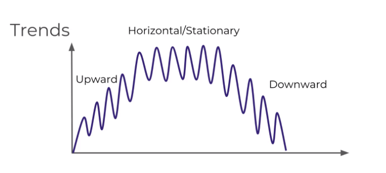
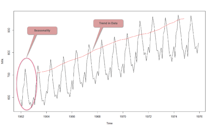
• Trend : Trend is a pattern in data that shows the movement of a series to relatively higher or lower values over a long period of time. In other words, a trend is observed when there is an increasing or decreasing slope in the time series. Trend usually happens for some time and then disappears, it does not repeat. For example, some new song comes, it goes trending for a while, and then disappears. There is fairly any chance that it would be trending again.

A trend could be :

1. Uptrend: Time Series Analysis shows a general pattern that is upward then it is Uptrend.
2. Downtrend: Time Series Analysis shows a pattern that is downward then it is Downtrend.
3. Horizontal or Stationary trend: If no pattern observed then it is called a Horizontal or stationary trend.

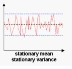
• Stationarity : A time series is said to be stationary, when it’s statistical properties do not change over time. That is, it has constant mean and variance, and covariance is independent of time. Ideally, we need to have a stationary time series for modelling. The reason for this is, when we try to make predictions on a time series, the statistical properties (mean, variance and correlation) of the time series should not be different than the ones currently observed. If the time series was non-stationary, making models and predictions on these properties would not give us an accurate result, as these properties would have changed.

• Seasonality : Seasonality is a characteristic of a time series in which the data experiences regular and predictable changes that recur every calendar year. Any predictable fluctuation or pattern that recurs or repeats over a one-year period is said to be seasonal.Seasonality refers to predictable changes that occur over a one-year period in a business or economy based on the seasons including calendar or commercial seasons. For example, The sudden increase in sales during holiday seasons are seasonal . they are bound to happpen, The sudden decrease in the temperature during winters is seasonal.

Image credit

• Cyclic effects :Cyclical variations are due to the ups and downs recurring after a period from time to time. These are due to the business cycle and every organization has to phase all the four phases of a business cycle some time or the other. Prosperity or boom, recession, depression, and recovery are the four phases of a business cycle.To understand if the time series is cyclic there are few statistical testsbut the most useful information here would be a little knowledge of the domain or the organisation. For example, there is a sudden sales drop in a company due to economic recession and this information will not be seen in the data.

• Random Walk : A type of time series where values tend to persist overtime and the difference between periods are simply white noise.

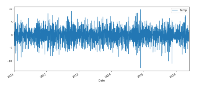
• White Noise : White noise is a special type of time series where the data does not follow a pattern.. If no pattern is seen we cannot consider the data having white noise.

In order to check if a series is white noise there are few conditions to be met :

1. The time series should have constant mean and constant variance.

2. should not have any correlation with any period. That means the time series should not be correlated with any number of lags.

Decomposition models in Time series

When you test if a time series's seasonality you will have to understand a term called decomposition . A decomposition is a a statistical task that deconstructs a time series into several components, each representing one of the underlying categories of patterns. The objective is to estimate and separate the four types of variations and to bring out the relative effect of each on the overall behavior of the time series. In other words decompostion is where we split the time series into 3 effects such as :

1. Trend : Pattern throughout the time series.
2. Seasonal : Cyclic effects throughout the time series .
3. Residual : Errors in the prediction.

The simplest type of decomposition is called Naive decomposition There are two approaches in the naive decomposition. such as :

• Additive Model : For any time period the observed value is the sum of the trend, seasonal and residual.

Observed = trend + seasonal + residual

• Multiplicative Model : for any time period the observed value is the product of trend, seasonal and residual.

Observed = trend x seasonal x residual

Model types in Time series

There are two types of time series models such as :

The classical time series models are as below :

1. ARIMA Family : The ARIMA family of models is a set of smaller models that can be combined. Each part of the ARMIA model can be used as a stand-alone component, or the different building blocks can be combined. When all of the individual components are put together, you obtain the SARIMAX model. You will now see each of the building blocks separately. Under ARIMA Familye there are few algorithms which are widely used . the list of algorithms are as follows :

• Autoregression(AR) : Autoregression is the first building block of the SARIMAX family. You can see the AR model as a regression model that explains a variable’s future value using its past (lagged) values. The order of an AR model is denoted as p, and it represents the number of lagged values to include in the model. The simplest model is the AR(1) model: it uses only the value of the previous timestep to predict the current value. The maximum number of values that you can use is the total length of the time series (i.e. you use all previous time steps).

• Moving average (MA) : The Moving Average is the second building block of the larger SARIMAX model. It works in a comparable way to the AR model: it uses past values to predict the current value of the variable.The past values that the Moving Average model uses are not the values of the variable. Rather, the Moving Average uses the prediction error in previous time steps to predict the future. This sounds counter-intuitive, but there is a logic behind it. When a model has some unknown but regular external perturbations, your model may have a seasonality or other pattern in the error of the model. The MA model is a method to capture this pattern without even having to identify where it comes from. The MA model can use multiple steps back in time as well. This is represented in the order parameter called q. For example, an MA(1) model has an order of 1 and uses only one time step back.

• Autoregressive moving average (ARMA): The Autoregressive Moving Average, or ARMA, model combines the two previous building blocks into one model. ARMA can therefore use both the value and the prediction errors from the past.ARMA can have different values for the lag of the AR and MA processes. For example an ARMA(1, 0) model has an AR order of 1 ( p = 1) and an MA order of 0 (q=0). This is actually just an AR(1) model. The MA(1) model is the same as the ARMA(0, 1) model. Other combinations are possible: ARMA(3, 1) for example has an AR order of 3 lagged values and uses 1 lagged value for the MA.

• Autoregressive integrated moving average (ARIMA) :The ARMA model needs a stationary time series. As you have seen earlier on, stationarity means that a time series remains stable. You can use the Augmented Dickey-Fuller test to test whether your time series is stable and apply differencing if it is not the case. The ARIMA model adds automatic differencing to the ARMA model. It has an additional parameter that you can set to the number of times that the time series needs to be differenced. For example, an ARMA(1,1) that needs to be differenced one time would result in the following notation: ARIMA(1, 1, 1). The first 1 is for the AR order, the second one is for the differencing, and the third 1 is for the MA order. ARIMA(1, 0, 1) would be the same as ARMA(1, 1).

• Seasonal autoregressive integrated moving-average (SARIMA):SARIMA adds seasonal effects into the ARIMA model. If seasonality is present in your time series, it is very important to use it in your forecast. SARIMA notation is quite a bit more complex than ARIMA, as each of the components receives a seasonal parameter on top of the regular parameter. For example, let’s consider the ARIMA(p, d, q) as seen before. In SARIMA notation, this becomes SARIMA(p, d, q)(P, D, Q)m. m is simply the number of observations per year: monthly data has m=12, quarterly data has m=4 etc. The small letters (p, d, q) represent the non-seasonal orders. The capital letters (P, D, Q) represent the seasonal orders.

• Seasonal autoregressive integrated moving-average with exogenous regressors (SARIMAX) :The most complex variant is the SARIMAX model. It regroups AR, MA, differencing, and seasonal effects. On top of that, it adds the X: external variables. If you have any variables that could help your model to improve, you could add them with SARIMAX.

2. Smoothing : Exponential Smoothing is a basic statistical technique that can be used to smoothen out time series. Time series patterns often have a lot of long term variability, but also short term (noisy) variability. Smoothening allows you to make your curve smoother so that long term variability becomes more evident and short term (noisy) patterns are removed.

Interpreting a Time Series Forecasting model